Code: https://github.com/raymondchua/simple_successor_features

1. Introduction

Deep Reinforcement Learning plays a crucial role in ensuring that intelligent systems can be relied upon to navigate complex and non-stationary environments. However, learning representations that are robust towards forgetting and interference remains a challenge.

Successor Features (SFs) offers a promising solution. However, learning SFs directly from complex, high-dimensional inputs, such as pixels, can lead to representation collapse, where the representations fail to capture key features in the data.

In this blogpost, we introduce our new approach — Simple Successor Features (Simple SFs) — a streamlined, efficient way to learn SFs directly from pixels without requiring pre-training or the use of complex auxiliary losses. Our method not only prevents representation collapse but also demonstrates superior performance in mitigating interference, and to a lesser extent, forgetting. Simple SFs achieve these results in continual reinforcement learning across 2D and 3D environments as well as complex continuous control tasks in Mujoco.

2. What are Successor Features exactly?

In Reinforcement Learning, an agent’s goal is to learn an optimal behavior (commonly known as policy function \(\pi\)) that corresponds to maximizing cumulative rewards. This is done by learning a Q-value function that estimates the future rewards for each state-action pair[1]. However, one challenge with this approach is that it can be hard to generalize knowledge across tasks, especially when the environment dynamics or the reward structure changes.

Just to give a short history, SFs are an extension of Successor Representations (SRs), which were initially developed to generalize across tasks by focusing on the environment transition dynamics [2]. SRs rely on tabular basis representation —a lookup table that stores each state individually which limits their scalability. SFs are a distributed, function-approximation variant of SRs, allowing replacing the tabular basis representation with a basis features vector, making them more suitable for high-dimensional inputs, such as pixels[3].

Just like SRs, we can decompose the Q-value function into two distinct components:

Successor Features \(( \psi )\): These capture the expected occupancy of each state, essentially providing a predictive map on where the agent might end
Task encoding \((\boldsymbol{w})\): Combined with the basis features, this component helps predict the reward value of a given state.

Mathematically, this means that for each state-action pair (s,a) can be defined as the linear combination of \(\psi(s,a)\) and \(\boldsymbol{w}\):

\[\begin{align}Q(s,a) = \psi(s,a)^{\intercal}\boldsymbol{w}\end{align}\]

3. Challenges of learning Successor Features from Pixels

In SRs, the tabular basis representations are usually pre-defined, such as using information about the spatial location of the agent to design this representation, which can also be adapted for basis features in SFs. However, in the scenario that the basis features have to be learned from high-dimensional inputs, such as pixels, things start to become tricky.

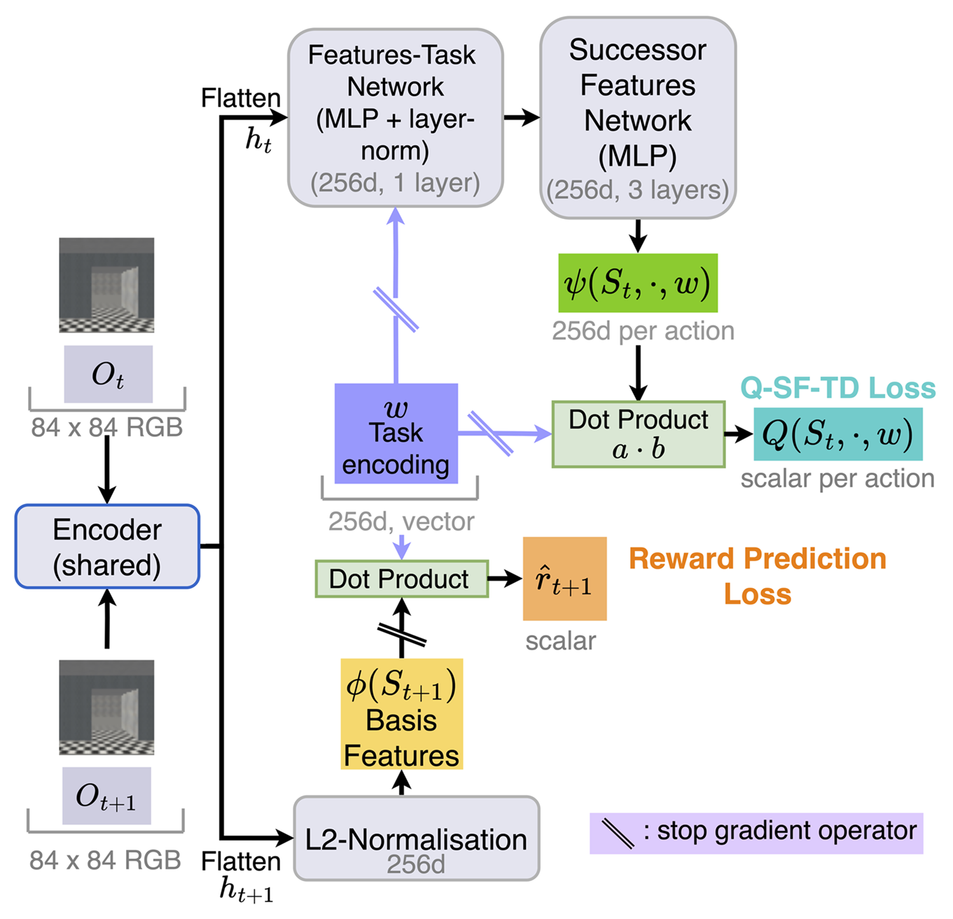
The core learning mechanism for the basis features \(\phi \in \mathbb{R}^{n}\) and SFs \(\psi \in \mathbb{R}^n\) is the SF-Temporal Difference (SF-TD) learning rule, which updates the successor features based on the agent’s transitions. The SF-TD loss is defined as follows:

\[\begin{align}L_{\phi, \psi} = \frac{1}{2} \left \| \phi(S_{t+1}) + \gamma {\psi}(S_{t+1}, a, \boldsymbol{w})) - \psi(S_{t},A_{t}, \boldsymbol{w}) \right \|^2\end{align}\]

where action \(a \sim \pi(S_{t+1})\) and \(\gamma \in [0,1]\) is the discount factor. We consider each transition to be \((S_t, A_t, S_{t+1}, R_{t+1})\), where \(S_t\) is the state at time-step \(t\), \(A_t\) is the action at time-step \(t\), \(S_{t+1}\) is the next state at time-step \(t+1\) and \(R_{t+1}\) is the reward at time-step \(t+1\).

When learning both the basis features \(\phi\) and the SFs \(\psi\) concurrently, this optimization can lead to representation collapse—where the learned features lose their discriminative characteristics across different states. This collapse occurs because the loss function is minimized if both \(\phi(\cdot)\) and \(\psi(\cdot)\) converge to constants across all states \(S\). Specifically, this happens when \(\phi(\cdot) = c_1\) and \(\psi(\cdot) = c_2\) with \(c_1 = (1-\gamma)c_2\).

For a more detailed proof, See section 3.4 in the paper.

To address this issue of representation collapse, some previous approaches have introduced pretraining [4] or auxiliary losses like reconstruction [5] and orthogonality [6] constraints. While these methods can help maintain feature diversity, they often add significant computational complexity. In contrast, our approach—Simple Successor Features (Simple SFs) —achieves similar resilience against collapse without requiring these additional components, as we discuss next.

4. Simple SFs: A New Approach

A key insight in designing Simple SFs is that the basis features \(\phi\) should not collapse to a constant, as this would allow the loss in Eq. 2 to be minimized trivially, leading to representation collapse. To address this, rather than directly optimizing Eq. 2, we leverage the definition in Eq. 1 and instead optimize the following losses:

Reward prediction loss guides the task encoding vector \(\boldsymbol{w}\) to capture reward-relevant information from the environment. Here, the basis features \(\phi\) are treats as a constant:

\[\begin{align}L_{\boldsymbol{w}} = \frac{1}{2}\left \| R_{t+1} - \overline{\phi}(S_{t+1})^\top \boldsymbol{w} \right \|^2\end{align}\]

Q-SF-TD loss allows the SFs \(\psi\) to be learned using a Q-learning like loss, treating the task encoding vector \(\boldsymbol{w}\) as a constant learning only the SFs \(\psi\):

\[\begin{align}L_{\psi} = \frac{1}{2}\left \| \hat{y} - \psi(S_t, A_t, \boldsymbol{w})^{\top}\boldsymbol{w} \right \|^2\end{align}\]

By optimizing these losses, we ensure that the task encoding \(\boldsymbol{w}\) effectively captures reward-relevant information, while the SFs \(\psi\) are learned in a stable way without collapse, allowing Simple SFs to learn effectively from high-dimensional inputs, such as pixels.

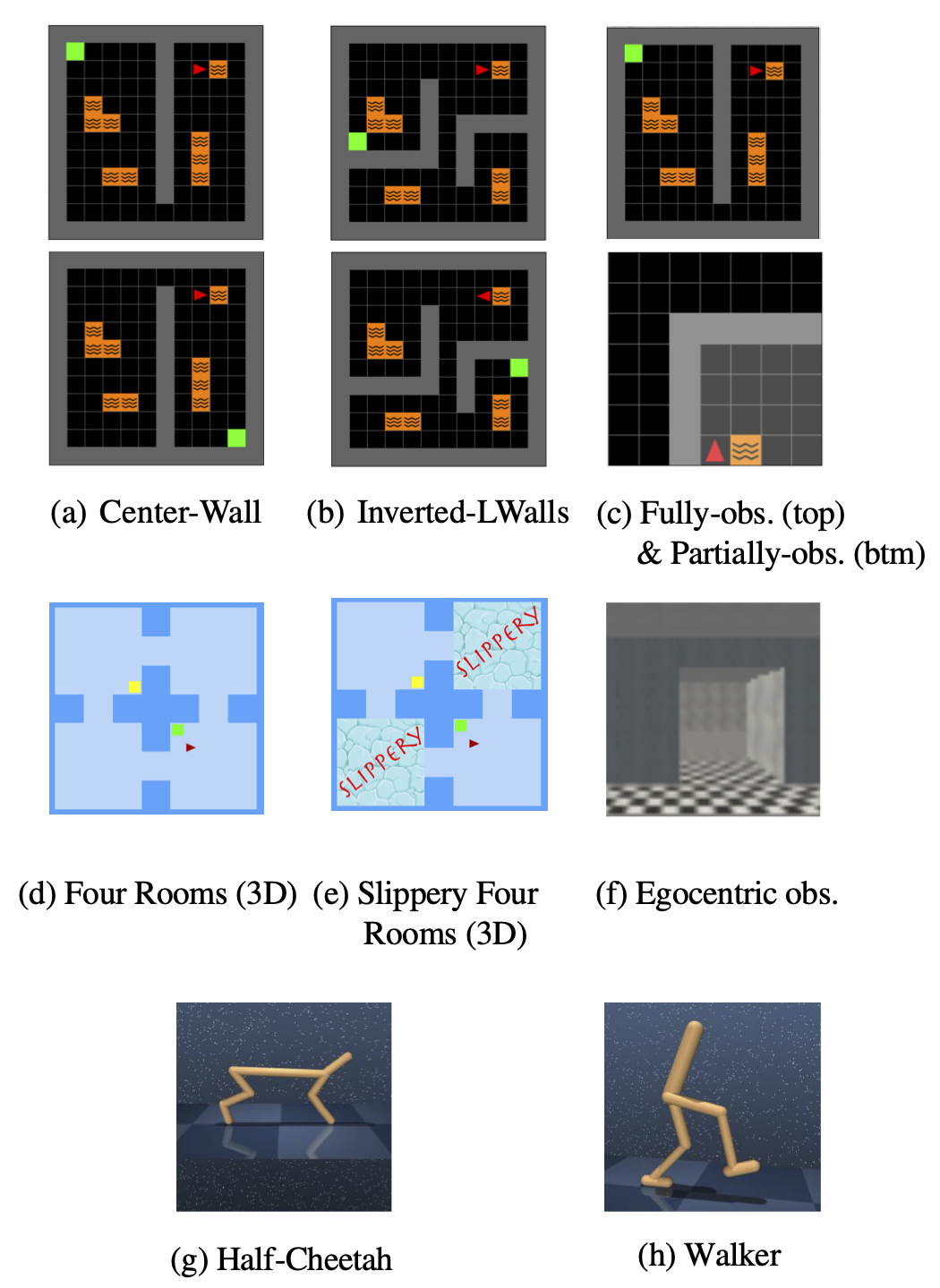
Figure 1: Architecture for Simple SFs for discrete actions

5. Environments

We evaluated our approach using 2D Minigrid, 3D Four Rooms environment and continuous control tasks in Mujoco, all within a continual learning setting. Agents are presented two tasks sequentially and then are re-exposed the same set of tasks in the same sequence a second time. All the studies were conducted exclusively using pixel observations as the primary motivation of this work is to address representation collapse when learning from high-dimensional pixel inputs.

The baseline models that we compare our approach to are Double Deep Q-network agent [7] or DDPG (for continuous actions) [8], and agents learning SFs with constraints on their basis features \(\phi\), such as reconstruction loss [5], orthogonal loss [6], and unlearnable random features[6]. We also compare with an agent that learns SFs using a pre-training regime which does not require rewards from the environment [4].

Figure 2: Environments used in our study. **(a-c):** We examined both egocentric (partially observable) and allocentric (fully observable) pixel observations in 2D Minigrid environments. Tasks included changes in reward locations (Inverted-L Walls) and combined changes in rewards and transition dynamics (Center-Wall). **(d-f):** Egocentric observations in a 3D Four Rooms environment, where the reward alternates between +1 for green and -1 for yellow in the first task, and -1 for green and +1 for yellow in the second task. **(e):** A slippery variant of the 3D Four Rooms environment, where selected agent actions are occasionally replaced by random actions based on a predefined slip probability. **(g-h):** Mujoco continuous control tasks, where agents either run forward and then backward, run forward at an increased speed in the second task, or switch from Half-Cheetah to Walker while being rewarded for running forward in the second task.

6. Results for 2D Minigrid and 3D Miniworld

2D and 3D Mazes results — Figure 3: Continual Reinforcement Learning Evaluation with pixel observations in 2D Minigrid and 3D Four Rooms environment. *Replay buffer resets at each task transitions to simulate drastic distribution shifts*: Agents face two sequential tasks (Task 1 & Task 2), each repeated twice (Exposure 1 & Exposure 2). **(a-c):** The total cumulative returns accumulated during training. Overall, our agent, Simple SF (orange), shows notable superiority and exhibited better transfer in later tasks over both DQN (blue) and agents with added constraints. Importantly, constraints like reconstruction and orthogonality on basis features can impede learning.

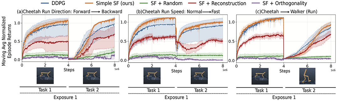
7. Results for Mujoco Continuous Control Tasks

Mujoco results — Figure 4: Continual Reinforcement Learning results using pixel observations in Mujoco environment across 5 random seeds. *Replay buffer resets at each task transitions to simulate drastic distribution shifts.* we started with the half-cheetah domain in Task 1 where agents were rewarded for running forward. We then introduced three different scenarios in Task 2: **(a)** agents were rewarded for running backwards, **(b)** running faster, and, in the most drastic change, **(c)** switching from the half-cheetah to the walker domain with a forward running task. To ensure comparability across these diverse scenarios, we normalized the returns, considering that each task has different maximum attainable returns per episode. We did not evaluate APS (Pre-train) here because it struggles in the Continual RL setting, even in simpler environments such as the 2D Minigrid and 3D Miniworld.

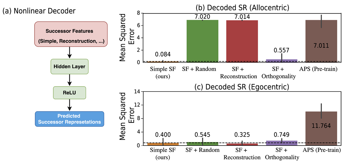
8. How effectively can Successor Features be decoded into Successor Representations?

Can our approach learn Successor Features that capture the environment’s transition dynamics in the same way as Successor Representations [2]? To investigate, we created a simple non-linear decoder (as shown in Figure (a) below) that takes the learned SFs as inputs and compares the predicted outcomes with analytically computed SRs. The SRs are calculated using:

\[\begin{align}\text{SR} = (I - \gamma T)^{-1}\end{align}\]

where \(T\) is the transition probability matrix derived from the same policy used the SFs. We used mean squared error (MSE) to measure the similarity between the SFs and the predicted SRs in both egocentric and allocentric observations, using the Center-Wall environment after training the non-linear decoder. Results show that the SFs learned using our approach consistently achieve lower MSE compared to baseline models (Figure (b and c) below).

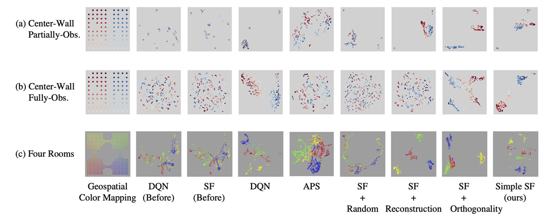
SR Decoder — Figure 5: **(a)** Architecture of the non-linear decoder model. **(b-c)** Comparison of the Mean Squared Error (MSE) between the learned SFs and the predicted SRs in the Center-Wall environment. Our approach consistently achieves lower MSE compared to baseline models, indicating that our SFs capture the environment's transition dynamics effectively.

9. How well do similar Successor Features that are proximate in neural space correspond to proximity in physical space?

Using UMAP, we visualise the Successor Features in 2D space for the Center-Wall environment in both egocentric (partially observable) and allocentric (fully-observable) scenarios, as well as the 3D Four Rooms environment with egocentric observations. A geospatial color mapping is applied to the SFs to examine whether SFs that are close in physical space exhibit similar representations in neural space.

The visualisation below shows that our approach consistently produces well-organized clusters in all the scenarios, unlike other baseline models. Notably, while some approaches using reconstruction or orthogonality constraints may yield well-clustered SFs, these clusters do not always translate into effective policy learning.

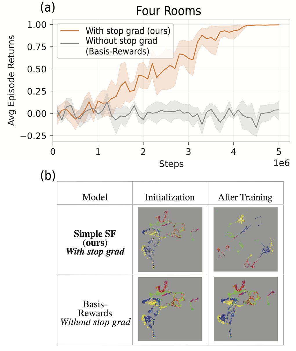
UMAP results — Figure 6: UMAP visualisation of Successor Features in 2D space for the Center-Wall environment in both egocentric (partially observable) and allocentric (fully-observable) scenarios, as well as the 3D Four Rooms environment with egocentric observations. A geospatial color mapping is applied to the SFs to examine whether SFs that are close in physical space exhibit similar representations in neural space.

10. How important is the stop-gradient operator for effective learning?

In a sparse rewards environment, such as the 2D Minigrid and 3D Four Rooms environments, learning the basis features \(\phi\) and the task encoding vector \(\boldsymbol{w}\) concurrently using the Reward prediction loss (Eq. 3) can be challenging. A possible issue is that the basis features \(\phi \rightarrow \vec{0}\) , minimizing the loss but resulting in ineffective learning. Additionally, we want the task encoding vector \(\boldsymbol{w}\) to capture information solely about the rewards, without being influenced by the basis features \(\phi.\) To address this, we apply a stop-gradient operator on the basis features during learning with the Reward prediction loss (Eq. 3).

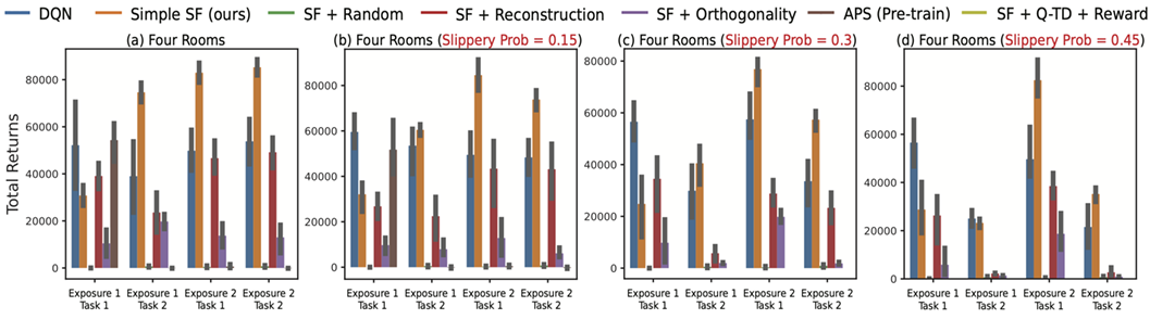
11. How robust are the Successor Features to stochasticity within the environment?

To evaluate the robustness of SFs, we introduced stochasticity into the environment by applying a predetermined “slippery” probability, where agents’ selected actions are occasionally replaced with alternative random actions. This study was conducted across varying degrees of stochasticity (0.15, 0.3, and 0.45). Results show that our approach consistently demonstrates better learning efficiency compared to other baseline methods.

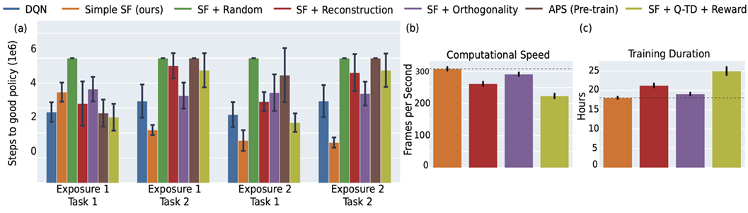
Stochasticity analysis — Figure 8: Analysis of the robustness of SFs to stochasticity within the environment, using a predetermined *slippery* probability, resulting in actions being occasionally replaced with alternative random actions.

12. How efficient is our approach relative to other methods?

To study the efficiency of our approach, we examined various metrics, such as time taken for the agent to learn a good policy, the frames per second during backpropagation, and the overall time required for the agent to complete sequential tasks. As expected, approaches that use additional objectives, such as reconstruction or orthogonality constraints on the basis features \(\phi\), require more computational resources.

Efficiency analysis — Figure 9: Analysis of the efficiency of our approach relative to other methods.

13. Conclusion

In this blogpost, we introduced Simple Successor Features (Simple SFs), a streamlined approach to learning SFs directly from pixel observations without relying on complex auxiliary objectives such as reconstruction or orthogonality constraints. By focusing on an efficient and straightforward design, Simple SFs successfully mitigate issues like representation collapse and interference, achieving robust learning performance in dynamic, high-dimensional environments. The simplicity of our approach not only reduces computational demands but also enhances scalability, making it a practical choice for continual learning tasks. These results highlight the potential of Simple SFs as a powerful yet efficient solution in environments where both adaptability and computational efficiency are critical.

14. References

[1] Sutton, Richard S. “Reinforcement learning: An introduction.” A Bradford Book (2018).

[2] Dayan, Peter. “Improving generalization for temporal difference learning: The successor representation.”Neural computation5.4 (1993): 613-624.

[3] Borsa, Diana, et al. “Universal successor features approximators.”arXiv preprint arXiv:1812.07626 (2018).

[4] Liu, Hao, and Pieter Abbeel. “Aps: Active pretraining with successor features.”International Conference on Machine Learning. PMLR, 2021.

[5] Machado, Marlos C., Marc G. Bellemare, and Michael Bowling. “Count-based exploration with the successor representation.”Proceedings of the AAAI Conference on Artificial Intelligence. Vol. 34. No. 04. 2020.

[6] Touati, Ahmed, Jérémy Rapin, and Yann Ollivier. “Does zero-shot reinforcement learning exist?.”arXiv preprint arXiv:2209.14935 (2022).

[7] Van Hasselt, Hado, Arthur Guez, and David Silver. “Deep reinforcement learning with double q-learning.”Proceedings of the AAAI conference on artificial intelligence. Vol. 30. No. 1. 2016.

[8] Lillicrap, T. P. “Continuous control with deep reinforcement learning.”arXiv preprint arXiv:1509.02971(2015).